SNooPy Example 1

This is a short example of how to fit lightcurves in SNooPy.

Here's the situation. You've got some data that is in an ASCII file that SNooPy understands (see the manual), let's say SN1981D.txt. This optical data was taken in some photometric system that is best described by the "standard" Landolt system with filters defined by Johnson and Morgan (hence we define them as Bs and Vs). The NIR data is close enough to the CSP NIR system that we just use 'J', 'H' and 'K'. Note that the times in the data file are in units of days relative to an arbitrary zero-point, which has no effect on the fitting other than the zero-point of date-related output parameters (like the time of B-band maximum). You can choose, JD, MJD, or even DJD (google it). First, we start up SNooPy and load in the text file.

% snpy
< Welcome message>

In[1]: s = get_sn('SN1981D.txt')

Now the data is associated with the supernova object, s. You can get a summary of the status so far.

In [2]: s.summary()
--------------------------------------------------------------------------------
SN  SN1981D
z = 0.006          ra= 50.65992         dec=-37.23272 
Data in the following bands: H,  K,  J,  Bs,  Vs,  
Fit results (if any):

Obviously, there are no fit results as we have not fit anything yet. But you can see the heliocentric redshift of the SN, the equitorial coordinates (ra, dec), and what filters there are. To get a feel for the data, try plotting it out:

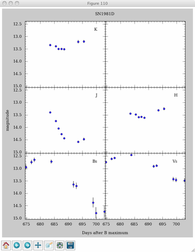
In[3]: s.plot()

which will open up a window and give you the following plot (this is the matplotlib default color scheme, PGPLOT is no longer supported):

SN1981D.lc.png

Each panel is the observed data in a different filter. The filters Bs and Vs are the "standard" Landolt system. The filters J, H, and K, are close enough to the Persson et al. (1998) system, which is also the CSP natural system. SNooPy can fit light-curves in the standard system BsVsRsIs using Jose Prieto's templates and calibration. But for the purposes of this example, we will fit Bs and Vs using the CSP natural B and V filters and let it handle the S-corrections. So, we can have a look at what restbands are being used to fit the observed bands and modify the ones we want:

In [4]: s.restbands
Out[4]: H -> H, K -> K, J -> J, Bs -> Bs, Vs -> Vs, 

In [5]: s.restbands['Bs'] = 'B'

In [6]: s.restbands['Vs'] = 'V'

In [7]: s.restbands
Out[7]: H -> H, K -> K, J -> J, Bs -> B, Vs -> V,

As you can see, the observed band Bs and Vs are now going to be fit with CSP B and V filters, respectively. SNooPy will do the S-corrections automatically as part of the fitting. If this SN were at high enough redshift, SNooPy would have chosen the redshifted CSP passbands that are closest to the observed passbands. You could override this choice in the same was as was done above. Now that the restbands are properly setup, we can do a fit:

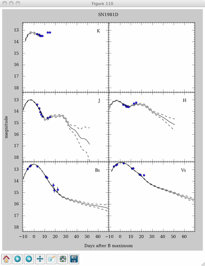
In[8]:  s.fit(['Bs','Vs','J','H'])

Simply specify which filters to fit (or omit the list to fit them all).

What actually happens: 1) SNooPy makes an initial fit to determine time of B-maximum, 2) initial k-corrections are determined from the Hsiao et al. (2007) SED templates, 3) another fit is made, this time including k-corrections, 4) the fit model is used to compute colors as a function of time, 5) improved k-corrections are computed, warping the Hsiao SED to match the observed colors, 6) a final fit is done with the color-matched k-corrections. What you see: the final fit plotted out.

SN1981D.lc_fit.png

Now, when we print the summary, there's more.

In [9]: s.summary()
--------------------------------------------------------------------------------
SN  SN1981D
z = 0.006          ra= 50.65992         dec=-37.23272 
Data in the following bands: H,  K,  J,  Bs,  Vs,  
Fit results (if any):
   Observed Vs fit to restbad V
   Observed Bs fit to restbad B
   EBVhost = 0.154  +/-  0.046
   Tmax = 679.389  +/-  0.286
   DM = 31.309  +/-  0.044
   dm15 = 1.212  +/-  0.074

For posterity, we can save all this information, along with the plots into a SNooPy file (my convention is to use the extension .snpy)

In [10]: s.save('SN1981D.snpy')

This file can later be loaded into SNooPy using the same function that was used to load the data: get_sn(). If you want to output the light-curve data and model that was fit, you can do:

In[11]: s.dump_lc()

That will create a whole bunch of files, two for each filter (data plus model).